

In this project, we aim to measure the influence of language on the number of views as one of the most important currencies in social media.
For this purpose, headlines from selected bloggers are loaded using the YouTube API and an attempt is made to classify them using LLM (GPT) as sensational, attention-seeking, ‘normal’, or meaningless.
In a second step, views loaded via the YouTube API are also to be predicted.
We want to show that sensational titles receive a significantly higher number of views – a critique that also comes from the authors themselves.
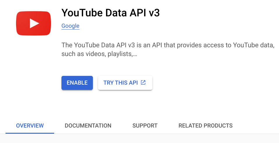
To download the title lists of a channel, a Google API3 key for YouTube is mandatory. This is free of charge. Beforehand, a project must be created at Google.
https://console.cloud.google.com/projectselector2/apis/dashboard?supportedpurview=project
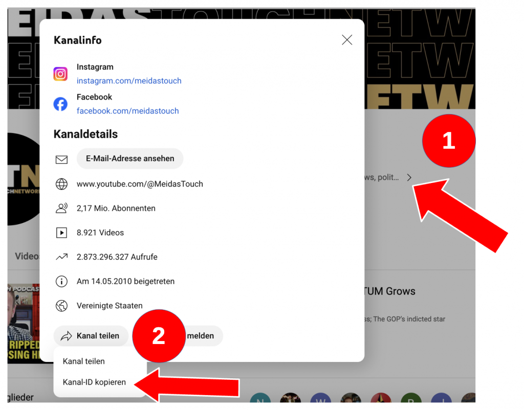
The actual download is performed by a Python script upon entering the channel_id. The latter can be extracted fromthe source of the respective YouTube channel by searching for “?channel_id“.
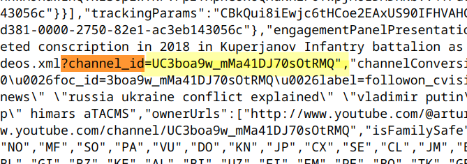
or go this way ….
With the following command, the required package is installed on the command line (bash) using pip (the package installer for Python).
# install google-api-python-client
pip install --upgrade google-api-python-client
Create a python script: youtube_get_channel.py
from googleapiclient.discovery import build
import os
Replace ‘YOUR_API_KEY’ with your actual YouTube Data API key
api_key = ‘enter your api key here’
youtube = build(‘youtube’, ‘v3’, developerKey=api_key)
Replace ‘CHANNEL_ID’ with the actual ID of the YouTube channel
from googleapiclient.discovery import build
import os

# Replace 'YOUR_API_KEY' with your actual YouTube Data API key
api_key = 'enter your api key here'
youtube = build('youtube', 'v3', developerKey=api_key)

# Replace 'CHANNEL_ID' with the actual ID of the YouTube channel
channel_id = 'UC3boa9w_mMa41DJ70sOtRMQ'
# Fetch the channel's uploads playlist ID
channel_response = youtube.channels().list(
    id=channel_id,
    part='contentDetails'
).execute()

uploads_playlist_id = channel_response['items'][0]['contentDetails']['relatedPlaylists']['uploads']

# Iterate through all videos in the uploads playlist
nextPageToken = None
while True:
    playlist_response = youtube.playlistItems().list(
        playlistId=uploads_playlist_id,
        part='snippet',
        maxResults=50,  # Adjust based on your needs
        pageToken=nextPageToken
    ).execute()

    for video in playlist_response['items']:
        video_id = video['snippet']['resourceId']['videoId']
        video_title = video['snippet']['title']

        # Fetch video statistics
        video_response = youtube.videos().list(
            id=video_id,
            part='statistics'
        ).execute()

        views = video_response['items'][0]['statistics']['viewCount']
        print(f'Title: {video_title}, Views: {views}')

    nextPageToken = playlist_response.get('nextPageToken')
    if not nextPageToken:
        break
# run the script
python3 ./youtube_get_channel.py > some_channel_name.out
NPL with R
2024 by Robert Kofler
NLP tasks: text preprocessing > feature extraction > sentiment analysis > and topic modeling.
Step 1: Text preprocessing
Theory:
Removal of punctuation, stop words, tokenization, and normalization of text (such as stemming or lemmatization). We use the tm package.
Common issues:
- generate correct csv w/ quoting and escaping and line ending!
- correct wrong encoding -> fix-encoding.py
- don’t use teams: no csv preview
- calculate views ratio (nb! div/0)
- make sure headlines are w/o !
install.packages("tm")
install.packages("SnowballC")
library(tm)

# Load data
# for NLP tasks: stringsAsFactors = FALSE
data <- read.csv("headlines.csv", stringsAsFactors = FALSE)

# show what we got.
str(data)

# Create a corpus
# a so-called Corpus ... is a representation of a collection of text documents.
corpus <- VCorpus(VectorSource(data$headline))

# Text Preprocessing
corpus <- tm_map(corpus, content_transformer(tolower))
corpus <- tm_map(corpus, removePunctuation)
# remove stop words “the”, “is” and “and”
corpus <- tm_map(corpus, removeWords, stopwords("english"))
# finde den Wortstamm (Porter's stemming algo)
# https://de.wikipedia.org/wiki/Porter-Stemmer-Algorithmus
Step 2: Feature Extraction
For text data to be used in machine learning models, it needs to be converted into a numeric format. The two common techniques are the Bag of Words and TF-IDF.
library(text2vec)

# Create a document-term matrix
dtm <- DocumentTermMatrix(corpus)

# Alternatively, create a TF-IDF matrix
tfidf <- weightTfIdf(dtm)
Step 3: Sentiment Analysis
Sentiment analysis can help determine the attitude or emotion of the text. We are using the syuzhet package.
NB! Latest developments in this area: Embedding with BERT model (Bidirectional Encoder Representations from Transformers (BERT)) -> this will be subject of 2025.
library(syuzhet)

# Get sentiment scores
sentiments <- get_nrc_sentiment(as.character(data$headline))
data <- cbind(data, sentiments)
Step 4: Themenerkennung / Topic Modeling
Die Themenerkennung wird verwendet, um abstrakte Themen innerhalb einer Sammlung von Dokumenten zu entdecken. Wir verwenden das topicmodels-Paket.
EXKURS:
topicmodels: An R Package for Fitting Topic Models
This article is a (slightly) modified and shortened version of Grün and Hornik (2011), published in the Journal of Statistical Software.
Topic models allow the probabilistic modeling of term frequency occurrences in documents. The fitted model can be used to estimate the similarity between documents as well as between a set of specified keywords using an additional layer of latent variables which are referred to as topics.
The R package topicmodels provides basic infrastructure for fitting topic models based on data structures from the text mining package tm. The package includes interfaces to two algorithms for fitting topic models: the variational expectation-maximization algorithm provided by David M. Blei and co-authors and an algorithm using Gibbs sampling by Xuan-Hieu Phan and co-authors.
library(topicmodels)

# Latent Dirichlet Allocation
# Estimate a LDA model using for example the VEM algorithm or Gibbs Sampling.
lda_model <- LDA(dtm, k = 3)  # k = number of topics

#Extract most likely terms or topics.
topics <- topics(lda_model)

#The function terms is a generic function which can be used to extract terms objects from various kinds of R data objects.
topic_terms <- terms(lda_model, 6)  # Get top 6 terms for each topic
Step 5: Machine Learning Models – Logistic Regression – glm()
Now we extracted features from text (like TF-IDF) to train a predictive models. Here we are going to use logistic regression.
# recoing of dependent variable in a binary form, threshold = MEDIAN
data$target <- ifelse(data$ratio_views_followers > median(data$ratio_views_followers), 1, 0)

# Fit a logistic regression model
model <- glm(data = train_data, target ~ abos + channelname + anger + anticipation + disgust + fear + joy + sadness + surprise + trust + negative + positive, family = "binomial")

summary(model)
Now interpret your model
What sentiment has a significat influence on view rate?
> summary(model)

Call:
glm(formula = target ~ anger + anticipation + disgust + fear +
    joy + sadness + surprise + surprise + trust + negative +
    channelname, family = "binomial", data = train_data)

Coefficients:
                                                  Estimate Std. Error z value Pr(>|z|)
(Intercept)                                       -3.45136    1.01911  -3.387 0.000708 ***
anger                                              0.10768    0.04222   2.550 0.010765 *
anticipation                                      -0.09657    0.03973  -2.431 0.015062 *
disgust                                            0.03100    0.05663   0.547 0.584070
fear                                               0.07827    0.03346   2.339 0.019313 *
joy                                               -0.04041    0.05090  -0.794 0.427281
sadness                                           -0.13956    0.04409  -3.165 0.001551 **
surprise                                          -0.15013    0.04367  -3.438 0.000587 ***
trust                                             -0.02420    0.03242  -0.747 0.455330
negative                                           0.11784    0.03454   3.411 0.000646 ***
channelnameATP Geopolitics                        18.81062  103.01116   0.183 0.855106
channelnameBBC News                                2.84145    1.01924   2.788 0.005307 **
channelnameBrian Tyler Cohen                       7.90615    1.03987   7.603 2.89e-14 ***
channelnameClimateScience - Solve Climate Change   7.00347    1.43744   4.872 1.10e-06 ***
channelnameCNN                                     4.18150    1.02098   4.096 4.21e-05 ***
channelnameEnvironment and Climate Change Canada  19.02910  134.32759   0.142 0.887347
channelnameeuronews                                2.04252    1.03436   1.975 0.048306 *
channelnameMilitary Summary                        7.18931    1.04585   6.874 6.24e-12 ***
channelnameRight Side Broadcasting Network         2.29647    1.05488   2.177 0.029481 *
channelnameSky News                                0.71018    1.18114   0.601 0.547663
channelnameThe Guardian                            3.06333    1.02519   2.988 0.002807 **
channelnameThe Independent                         0.05235    1.44035   0.036 0.971004
channelnameThe New York Times                      2.83837    1.01953   2.784 0.005369 **
channelnameThe Wall Street Journal                 2.73979    1.01951   2.687 0.007202 **
channelnameVICE News                               4.58010    1.02291   4.478 7.55e-06 ***
channelnameWar in Ukraine                          6.65964    1.05993   6.283 3.32e-10 ***
---
Signif. codes:  0 ‘***’ 0.001 ‘**’ 0.01 ‘*’ 0.05 ‘.’ 0.1 ‘ ’ 1

(Dispersion parameter for binomial family taken to be 1)

    Null deviance: 27504  on 19839  degrees of freedom
Residual deviance: 21135  on 19814  degrees of freedom
AIC: 21187

Number of Fisher Scoring iterations: 14